


Linseis – LSR Thermoelectrics
The Linseis LSR Thermoelectrics system is a versatile instrument designed to measure key properties of thermoelectric materials. It includes the ability to measure Seebeck coefficients, electrical resistivity, and thermal conductivity. The system is capable of assessing the performance of thermoelectric materials by calculating the figure of merit (ZT) and is suitable for both research and industrial applications, offering precise and reliable results for a wide temperature range.
Waste heat recovery / Thermoelectric generators (TEG) / Thermoelectric Peltier elements / Sensors / Thermoelectric pads / Thermoelectric modules

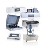
Measuring Devices for Thermoelectrics
Waste heat recovery / Thermoelectric generators (TEG) / Peltier elements / Sensors
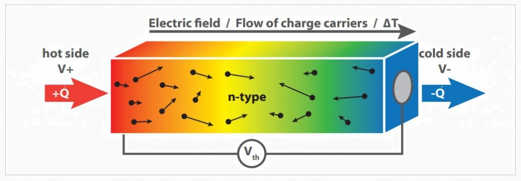
Seebeck, Peltier and Thomson effect
Thermoelectricity generally describes the reciprocal influence of temperature and electricity in a material and is based on three fundamental effects: the Seebeck effect, the Peltier effect, and the Thomson effect. The Seebeck effect was discovered in 1821 by Thomas J. Seebeck, a German physicist, and describes the occurrence of an electric field when a temperature gradient is applied in an electrically insulated conductor. The Seebeck coefficient (S) is defined as the quotient of negative thermoelectric voltage and temperature difference and is a purely material-specific quantity that is usually specified in the unit µV/K.
In view of the increasing scarcity of fossil fuels and the latest findings on global warming due to rising carbon dioxide emissions, the field of thermoelectricity has once again become the focus of public interest due to its effective use of waste heat. The aim is to utilize the waste heat from heat engines, such as cars or conventional power plants, by means of thermoelectric generators (TEGs) in order to increase their efficiency. However, efficient thermoelectric materials are also of great interest for cooling applications using the Peltier effect, such as the temperature control of temperature-critical components in lasers.
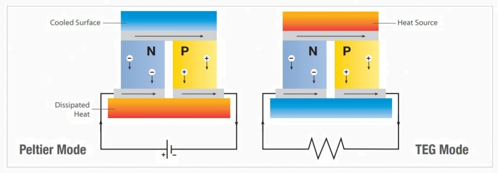
In the opposite case, this effect, known as the Peltier effect, causes a temperature gradient to appear when an external current is applied to the conductor. This phenomenon is due to the different energy levels of the conduction bands of the materials involved. When transferring from one material to another, the charge carriers must either absorb energy in the form of heat, causing the contact point to cool down, or they can release energy in the form of heat, causing the contact point to heat up.
The thermoelectric conversion efficiency of a material is usually compared using the dimensionless figure of merit ZT. This is calculated from the thermal conductivity, the Seebeck coefficient, and the electrical conductivity.
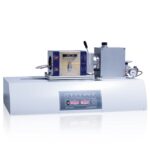
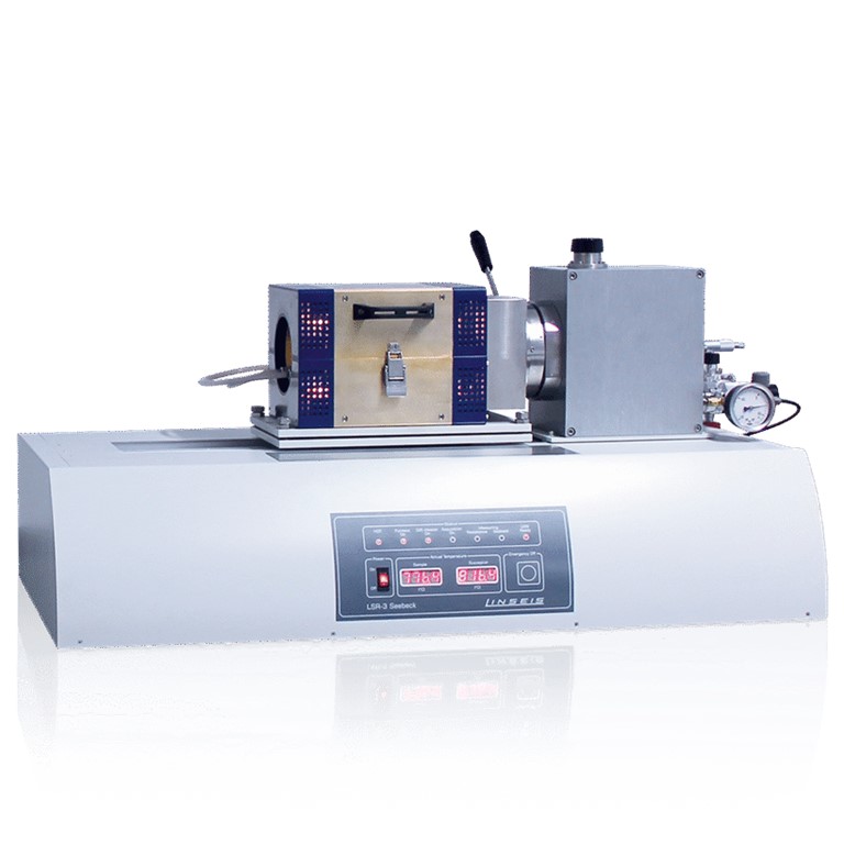
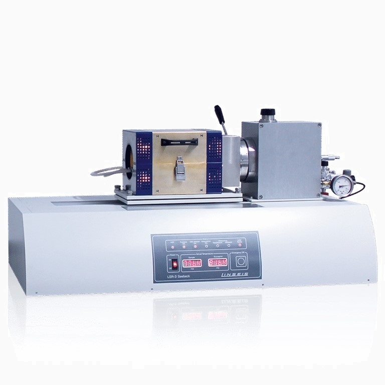
In order to support this development, an instrument for simple and extremely precise material characterization has been developed. The LINSEIS LSR-3 can determine both the Seebeck coefficient and the electrical resistance of a sample in a temperature range from –100°C to 1500°C.
Linseis Electrical Properties Series

IDEAL FOR
The LSR (Laser Flash System) series by Linseis is ideal for measuring thermoelectric properties of materials, including:
- Seebeck Coefficient: Determines the voltage generated due to a temperature gradient in a material.
- Electrical Conductivity: Measures how well a material can conduct electricity.
- Thermal Conductivity: Assesses the material’s ability to transfer heat.
- Figure of Merit (ZT): Evaluates the efficiency of thermoelectric materials by combining Seebeck coefficient, electrical conductivity, and thermal conductivity.
Applications:
- Thermoelectric Material Development: For power generation or cooling applications.
- Material Research: Understanding the thermal and electrical behavior of metals, semiconductors, and insulators.
- Energy Efficiency Studies: In renewable energy systems, waste heat recovery, and advanced material testing.
The LSR series is particularly suited for high-precision and high-temperature measurements, making it essential for R&D in energy-related materials.
FEATURES
MODEL |
TEG-TESTER |
|---|---|
| Sample size: | Round: ø 20 mm, 25 mm, 40 mm, 60 mm Rectangular: 20 mm x 20 mm, 25 mm x 25 mm, 40 mm x 40 mm Other sizes on request |
| Sample thickness: | up to 25 mm |
| Accuracy of thickness: | +/- 0.10 % at 50% tensile force +/- 0.25 % at 100% tensile force |
| Temperature range: | RT up to 300°C (on the hot side) / -20 °C up to 300 °C |
| Temperature accuracy: | 0.1°C |
| Voltage range: | 0 – 12 V (DC) |
| Accuracy of voltage: | 0.3 % |
| Voltage resolution: | 1.6 µV |
| Amperage: | 0-3 A (DC) |
| Current accuracy: | 0.3 % |
| Current resolution: | 1 µA |
| Heat dissipation: | up to 36 W |
| Rating: | Heat Flow Average Seebeck coefficient Average thermal conductivity Average module resistance Power output Conversion efficiency of the module |
| Reference block material: | Aluminium, brass, copper (others on request) |
| Temperature sensors: | Thermocouple type E |
| Clamping force: | 2 kN to 5 kN (electric drive) |
| Heating power: | 1.0 kW |
| Intracooler | |
| Cooling capacity: | 1.0 kW (10 °C) / 0.5 kW (-20 °C) |
| Pump capacity: | 27 l/min / 0.7 bar |
| Tank capacity: | 3.8 l up to 7.5 l |
| Refrigerant used: | R449 Liquid |
MODEL |
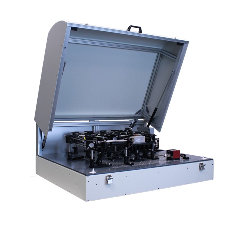
TF-LFA |
|---|---|
| Sample dimensions: | Any shape between 2mm x 2mm and 25mm x 25mm lateral size |
| Thin film samples: | 10nm up to 20μm* (depends on sample) |
| Temperature range: | RT, RT up to 200/500°C Sample holder for 4“ Wafer (only RT) |
| Measured properties: | Thermal conductivity Thermal diffusivity Thermal interface resistance Volumetric specific heat capacitiy Thermal effusivity |
| Options: | Anisotrophy: Measurement of cross-plane and in-plane thermal propertiesSample mapping: Scanning multiple positions of the sample pointwise or clusterwise. Mapping area: 10 mm² Stepsize: 50 μm Camera: |
| Atmosphere: | inert, oxidizing or reducing vaccuum up to 10E-4mbar |
| Diffusivity measuring range: | 0.01mm2/s up to 1200mm2/s (depends on sample) |
| Pump laser: | CW Laser (405 nm, 300 mW, modulations frequency up to 200 MHz) |
| Probe laser: | CW Laser (532 nm, 25 mW) |
| Photodetector: | Si Avalanche Photodetector, active diameter: 0.2 mm, bandwidth: DC – 400MHz |
| Power supply: | AC 100V ~ 240V, 50/60 Hz, 1 kVA |
| Software: | Included. Software package using multi-layer analysis for calculation of thermophysical properties |
| *Actual thickness range depends on sample | |
MODEL |
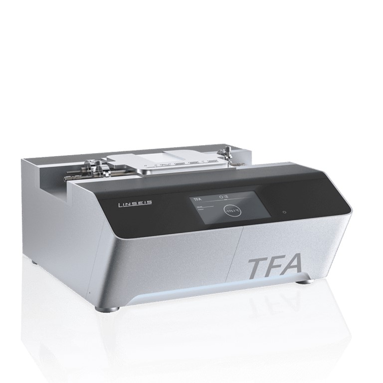
TFA – THIN FILM ANALYZER |
|---|---|
| Temperature range: | RT to 280°C -160°C to 280°C |
| Sample thickness: | From 5 nm to 25 µm (depending on sample) |
| Measuring principle: | Chip-based (pre-structured measuring chips, 24 pieces per box) |
| Separation techniques: | Among others: PVD (sputtering, vaporisation), ALD, spin coating, ink-jet printing and many more |
| Measured parameters: | Thermal conductivity (3 Omega) |
| Heat capacity | |
| Optional: | Electrical conductivity / specific resistance Hall constant / mobility / charge carrier density (electromagnet up to 1 T or permanent magnet with 0.5 T) |
| Vacuum: | ~10E-4mbar |
| Electronics: | Integrated |
| Interface: | USB |
| Measuring range | |
| Thermal conductivity: | 0.05 to 200 W/m∙K 3 Omega method, hot-strip method (in-plane measurement) |
| Electrical conductivity: | 0.05 to 1 ∙ 106 S/cm Van der Pauw four-probe measurement |
| Seebeck coefficient: | 5 to 2500 μV/K |
| Repeatability & Accuracy | |
| Thermal conductivity: | ± 3% (for most materials) ± 10% (for most materials) |
| Resistivity: | ± 3% (for most materials) ± 6% (for most materials) |
| Seebeck coefficient: | ± 5% (for most materials) ± 7% (for most materials) |
MODEL |
LSR-1 |
|---|---|
| Temperature range: | Basic unit: RT to 200°C Cryo option: -160°C to +200°C |
| Principles of measurement: | Seebeck coefficient measuring range: 0 to 2.5 mV/K – temperature gradient up to 10K Seebeck voltage measurement: range +-8 mV |
| Atmospheres: | Inert, reducing, oxidising, vacuum Helium gas with low pressure, recommended |
| Sample holder: | Integrated PCB board with primary and secondary heater |
| Sample size (Seebeck): | L: 8 mm to 25 mm; W: 2 mm to 25 mm; D: Thin film up to 2 mm |
| Sample size (resistance): | L: 18 mm to 25 mm; W: 18 mm to 25 mm; D: thin film up to 2 mm |
| Vacuum pump: | optional |
| Heating rate: | 0.01 – 100 K/min |
| Temperature accuracy: | ±1,5 °C oder 0,0040 ∙ | t | |
| Electrical resistance: | 10 nOhm |
| Thermal voltage: | 0.5 nV/K (nV = 10-9 V) |
MODEL |
LSR-3 |
|---|---|
| Temperature range: | Infrared oven: RT up to 800°C/1100°C Resistance oven: RT up to 1500°C Low temperature oven: -100°C to 500°C |
| Measurement method: | Seebeck coefficient: Static DC method / Slope method Electrical resistance: four-point measurement |
| Atmosphere: | Inert, reducing, oxidizing, vacuum Helium gas with low pressure recommended |
| Sample holder: | Vertical clamping between two electrodes Optional adapter for films and thin layers |
| Sample size (cylinder or rectangle): | 2 to 5 mm base area and max. 23 mm long up to a diameter of 6 mm and a length of max. 23 mm long |
| Sample size round (disc shape): | 10, 12.7, 25.4 mm |
| Measuring distance of the thermocouples: | 4, 6, 8 mm |
| Water cooling: | required |
| Measuring range Seebeck coefficient: | 1µV/K to 5000 µV/K (static direct current method) Accuracy ±7% / repeatability ±3.5% |
| Measuring range Electrical conductivity: | 0.01 to 2×10 5 S/cm Accuracy ±10% / repeatability ±5% |
| Current source: | Low drift current source from 0 to 160 mA (optional 220 mA) |
| Electrode material: | Nickel (-100 to 500°C) / Platinum (-100 to +1500°C) |
| Thermocouples: | Type K/S/C |
| * 5% for LSR including camera option | |
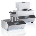
MODEL |
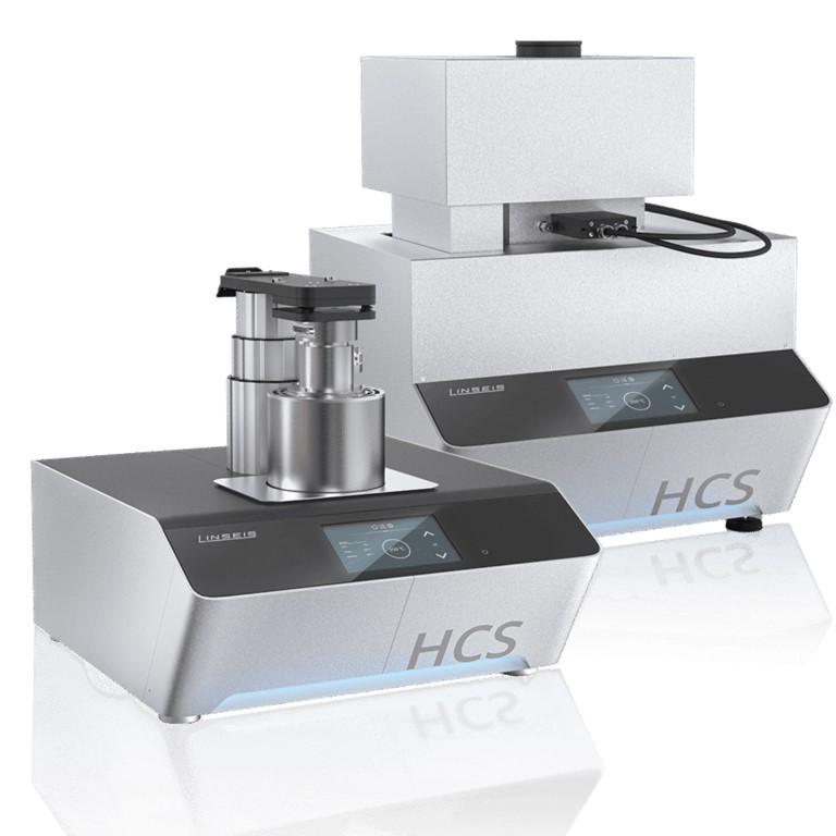
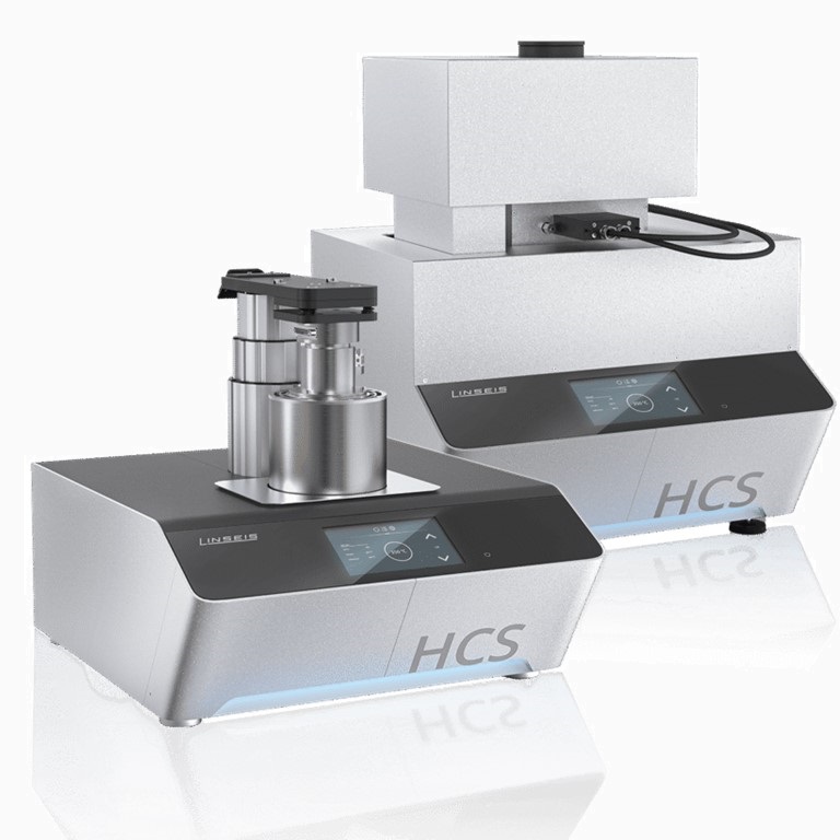
HCS 1 |
|---|---|
| Temperature range: | From LN2 up to 600°C in various versions -160°C (controlled cooling) -196°C (cooling) |
| Magnet: | Two permanent magnets with +/- 0.7T Diameter of the rod 120 mm for maximum uniformity (+/- 1% over 50mm) |
| Power supply: | DC 1nA up to 125mA (8 decades / compliance +/- 12V) |
| Voltage measurement: | DC low noise / low deviation 1μV up to 2500mV, 4 decades gain, digital resolution: 300pV |
| Sensors/ sample geometry: | – from 5 x 5 mm2 to 12.5 x 12.5 mm2, maximum sample height 3 mm – from 17.5 x 17.5 mm2 up to 25 x 25 mm2, maximum sample height 5 mm – from 42.5 x 42.5 mm2 up to 50 x 50 mm2, maximum sample height 5 mm – High temperature plate, 10 x 10mm2, max. sample height 2mm |
| Resistance range: | 10-4 up to 107(Ωcm) |
| Carrier concentration: | 107 up to 1021cm-3 |
| Mobility range: | 0.1 to 107(cm2/volt sec) |
| Atmospheres: | Vacuum, inert, oxidizing, reducing |
| Temperature accuracy: | 0.05°C |
MODEL |
HCS 10 |
|---|---|
| Temperature range: | From LN2 up to 600°C in various versions -160°C (controlled cooling) -196°C (quench cooling) |
| Magnet: | Electromagnet up to +/- 1 T variable DC field, pole diameter 76 mm, power supply 75A / 40V. Current reversing switch for bipolar measurement. Alternative AC option for an alternating magnetic field with ~1 T usable field, at a frequency of up to 0.1 Hz |
| Power supply: | DC 1nA up to 125mA (8 decades / compliance +/- 12V) AC 16 μA up to 20 mA and input impedance: >100 GigaOhm from 1 mHz to 100 kHz |
| Voltage measurement: | DC low noise / low deviation 1μV up to 2500mV, 4 decades gain, digital resolution: 300pV AC 20 nV up to 1V, variable integration times and gain |
| Sensors/ sample geometry: | – from 5 x 5 mm2 to 12.5 x 12.5 mm2, maximum sample height 3 mm – from 17.5 x 17.5 mm2 to 25 x 25 mm2, maximum sample height 5 mm – from 42.5 x 42.5 mm2 up to 50 x 50 mm2, maximum sample height 5 mm – High temperature plate, 10 x 10 mm2, maximum sample height 2 mm |
| Resistance range: | 10-4 up to 107(Ωcm) |
| Carrier concentration: | 107 up to 1021cm-3 |
| Mobility range: | 10-3 ~ 107cm2V-1s-1 |
| Atmospheres: | Vacuum, inert, oxidizing, reducing |
| Temperature accuracy: | 0.05°C |
MODEL |
HCS 100 |
|---|---|
| Temperature range: | RT up to 500°C |
| Magnet: | Magnet up to 0.5 T (AC or DC field) Multisegment Halbach configuration, inner diameter: 40mm, height: 98mm |
| Power supply: | DC 1nA up to 125mA (8 decades / compliance +/- 12V) AC 16 μA up to 20 mA and input impedance: >100 GigaOhm from 1 mHz to 100 kHz |
| Voltage measurement: | DC low noise / low deviation 1μV up to 2500mV, 4 decades gain, digital resolution: 300pV AC 20 nV up to 1V, variable integration times and gain |
| Sensors/ sample geometry: | Up to 10 x 10 mm2, maximum sample height 2.5 mm |
| Resistance range: | 10-5 up to 107(Ωcm) |
| Carrier concentration: | 107 up to 1022cm-3 |
| Mobility range: | 1 ~ 107cm2V-1s-1 |
| Atmospheres: | Vacuum, inert, oxidizing, reducing |
| Temperature accuracy: | 0.05°C |